Uncertainty and error in measurement

Scientists aim towards designing experiments that can give a “true value” from their measurements, but due to the limited precision in measuring devices, they often quote their results with some form of uncertainty.

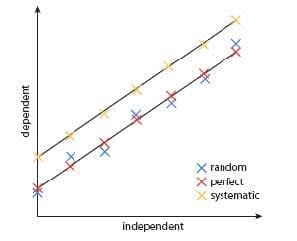
• Random errors are caused by:
  • the readability of the measuring instrument
  • the effects of changes in the surrounding such as temperature variations and air currents.
  • insufficient data
  • the observer misinterpreting the reading.
• Random errors make a measurement less precise, but not in any particular direction. They are expressed as an uncertainty range, such as $\rm 25.05 \pm 0.05~°C$.
• The uncertainty of an analogue scale is $\pm$ (half the smallest division).
• The uncertainty of a digital scale is $\pm$ (the smallest scale division).
• Systematic errors occur when there is an error in the experimental procedure.:
  For example:
  • measuring the volume of water from the top of the meniscus rather than the bottom,
  • heat loss due to insufficient insulation in thermal experiments another.
• Experiments are repeatable if the same person duplicates the experiment with the same results.
• Experiments are reproducible if several experimentalists duplicate the results.
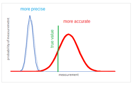
• The precision or reliability of an experiment is a measure of the random error. If the precision is high, then the random error is small.
• The accuracy of a result is a measure of how close the result is to some accepted or literature value If an experiment is accurate then the systematic error is very small.
  
• Random uncertainties can be reduced by repeating readings; systematic errors cannot be reduced by repeating measurements.
• Precise measurements have small random errors and are reproducible in repeated trials. Accurate measurements have small systematic errors and give a result close to the accepted value.
• If one uncertainty is much larger than others, the approximate uncertainty in the calculated result can be taken as due to that quantity alone.
• The experimental error in a result is the difference between the recorded value and the generally accepted or literature value.
• Percentage uncertainty $=$ (absolute uncertainty /measured value) $\times$ $100\%$
• Percentage error $=$ ((accepted value – experimental value)/ accepted value) $\times$ $100\%$

• Graphical techniques are an effective means of communicating the effect of an independent variable on a dependent variable and can lead to determination of physical quantities.
• The independent variable is the cause and is plotted on the horizontal axis. The dependent variable is the effect and is plotted on the vertical axis.
• Sketched graphs have labelled but unscaled axes, and are used to show qualitative trends, such as variables that are proportional or inversely proportional.
• Drawn graphs have labelled and scaled axes and are used in quantitative measurements.
• When drawing graphs:
  • Give the graph a title (always based on $y$ versus $x$) and label the axis with both quantities and units.
  • Use the available space as effectively as possible and use sensible scales – there should be no uneven jumps.
  • Plot all the points correctly.
  • Identify any points which do not agree with the general trend.
  • Think carefully about the inclusion of the origin. The point $(0, 0)$ can be the most accurate data point, or it can be irrelevant.
• You should be able to give a qualitative physical interpretation of a particular graph.
  

  The variables are proportional.	The variables are inversely proportional.

• A ‘best-fit’ straight line does not have to go through all the points but should show the overall trend.
• The equation for a straight line is:
  • $y = mx + c$.
  • $x$ is the independent variable,
  • $y$ is the dependent variable,
  • $m$ is the gradient.
  
  
• $m = \Delta y/ \Delta x$
  $m$ has units of $y /x$
• $c$ is the intercept on the vertical axis and has the units of $y$.
  
• A systematic error produces a displaced line.
• Random uncertainties lead to points on both sides of the perfect line.
  
• The gradient of a curve is given by the gradient of the tangent at that point.
  
• The process of assuming that the trend line applies between two points is called interpolation.
• A line is extrapolated when it is extended beyond the range of measurement.