In probability theory, there are many examples where the total number of outcomes is in fact infinite. No matter how much we try, there are just too many possibilities to consider. For example, consider the heights of grade $12$ students. If we really get precise, there are just too many possibilities to account for. Is a student really $\rm 172~cm$? Couldn’t we be more precise and measure the student as $\rm 172.1~cm$? Couldn’t we go further and be more precise and measure the student as $\rm 172.01~cm$ and so on? You get the point. When there are infinite cases to consider, this is called a continuous random variable.
Fortunately, if a large enough discrete sample size is considered, then we start to see a pattern emerge. We start to understand what the mean (average) is. We start to see how the cases are dispersed or deviated among the rest of the data set. That is to say, we know there will be some Grade $12$ students that are very tall, compared to their classmates. Likewise, there will be some Grade $12$ students that are very short compared to their classmates. However, when viewed as a large group, most students will be near the average and fewer and fewer students will deviate further away from the average. This leads us to the Normal Distribution. If $\rm X$ is normally distributed with mean $\mu$ and standard deviation $\sigma$, this is expressed as $\rm X\sim N(\mu,\sigma^2)$, where $\sigma^2$ is called the variance of $\rm X$ and is the standard deviation squared.
If $\rm X$ is normal distribution with mean $\mu$ and standard deviation $\sigma$, we can obtain a $\rm Z$ score which will tell us how many standard deviations away from the mean a particular value is. We do this using the following formula: $\rm Z=X−\mu\sigma$.
In the IB Approaches and Analysis SL course, a lot emphasis is placed on using the graphic display calculator to determine results.
Example: A large group of students took an exam. It was determined that the mean was $22$ points and the standard deviation was $3.5$ points. Determine the probability that a randomly selected student scored between $21$ and $24$ points inclusively.
Explanation: Graphically this is shown below:
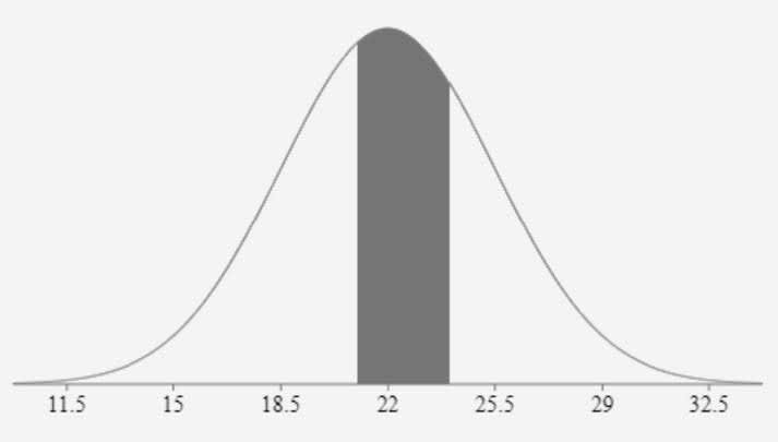
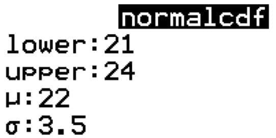
The area under the entire curve is $1$. So what is the area of the shaded region? The graphic display calculator makes this easy to determine. Using the normalcdf option in the dist command:
![]()
Thus, the probability is $0.329$. There is a $32.9\%$ chance that a randomly selected student scored between $21$ and $24$ points inclusively.