In the previous chapter, tangent lines were discussed in depth. Tangent lines will also play an important role in this chapter as we will be discussing specific tangent lines; those that have slopes of zero. Consider the cubic polynomial shown below:
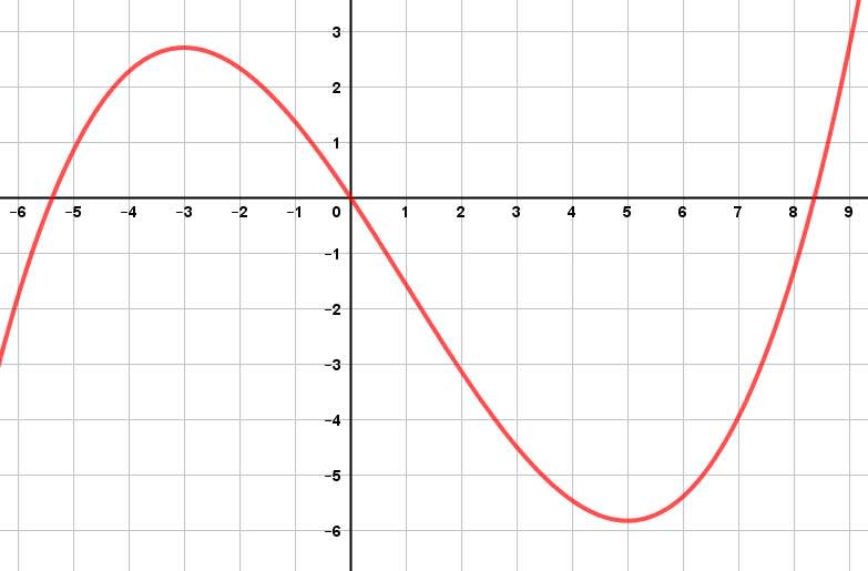
It is clear there is a local maximum, perhaps around $x=3$, and a local minimum, perhaps around $x=5$. These can be thought of as the “top of a hill” or “bottom of a valley”. Wherever a tangent line would be parallel to the x-axis, then the slope of these tangent lines, or derivatives, would be equal to zero. This is the underlying concept behind this chapter. There are many applications that we will examine in this chapter discussing maximums and minimums. Whether it is minimizing the surface area of a can or maximizing its volume, determining derivatives and equating them to zero will be of the utmost importance.
Example: Determine the coordinates of the local maximum and local minimum of:
$f(x)=\dfrac{1}{3}x^3−\dfrac{1}{2}x^2−6x+2$
Explanation: Any local max or mins occur where $f′(x)=0$. Therefore:
$f′(x)=x^2−x−6=0$
$\Rightarrow (x−3)(x+2)=0$
$\Rightarrow x=3$, $x=−2$
Therefore, the coordinates of any local max or min are given by:
$f(3)=9−\dfrac{9}{2}−18+2=−\dfrac{23}{2}$
$\Rightarrow \left(3,−\dfrac{23}{2}\right)$$f(−2)=−\dfrac{8}{3}−2+12+2=\dfrac{28}{3}$
$\Rightarrow \left(−2,\dfrac{28}{3}\right)$
Note: We do not necessarily know which point is the maximum and which point is the minimum. Such a concept is beyond the scope of this course.